1Learning Outcomes
Use laundry as an analogy to understand pipelined architectures.
Compare latency and throughput of sequential and pipelined architectures.
Understand that pipelining improves performance by increasing instruction throughput, in contrast to decreasing the execution time of an individual instruction. Instruction throughput is the important metric because real programs execute billions of instructions.
🎥 Lecture Video
The concept of pipelining will increase our compute throughput. Before we jump into our RISC-V pipeline, let’s first start with a real-life example of laundry. Anyone who has done a lot of laundry has intuitively used pipelining. The four steps of laundry are shown in Figure 1:
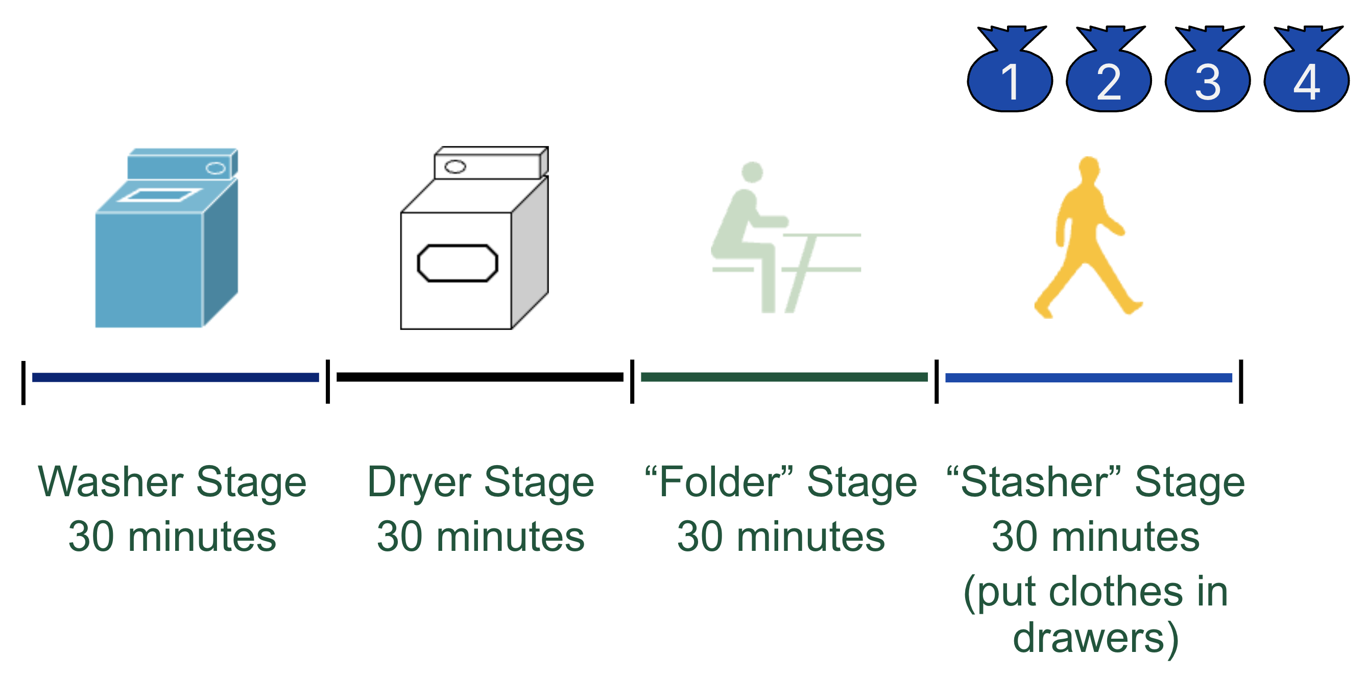
Figure 1:Laundry analogy.
Washer Stage (30 minutes). Place one dirty load of clothes in the washer.
Dryer Stage (30 minutes). When the washer is finished, place the wet load in the dryer.
“Folder” Stage (30 minutes). When the dryer is finished, place the dry load on a table and fold.
“Stasher” Stage (30 minutes). When folding is finished, put clothes in drawers.
Suppose our laundry benchmark task involves four people in a laundromat, or shared laundry room[1], who all need to do their laundry on a Sunday evening. In Figure 1, each person is denoted by a laundry bag with their number (1 through 4).
2Sequential Laundry
Consider a sequential approach to using laundry, where only one person can use the room at a time,[2] as shown in Figure 2. Person 1 starts at 6pm and finishes all four steps at 8pm; then, Person 2 starts and finishes 8-10pm, followed by Person 3, and finally Person 4, who doesn’t finish until 2am.
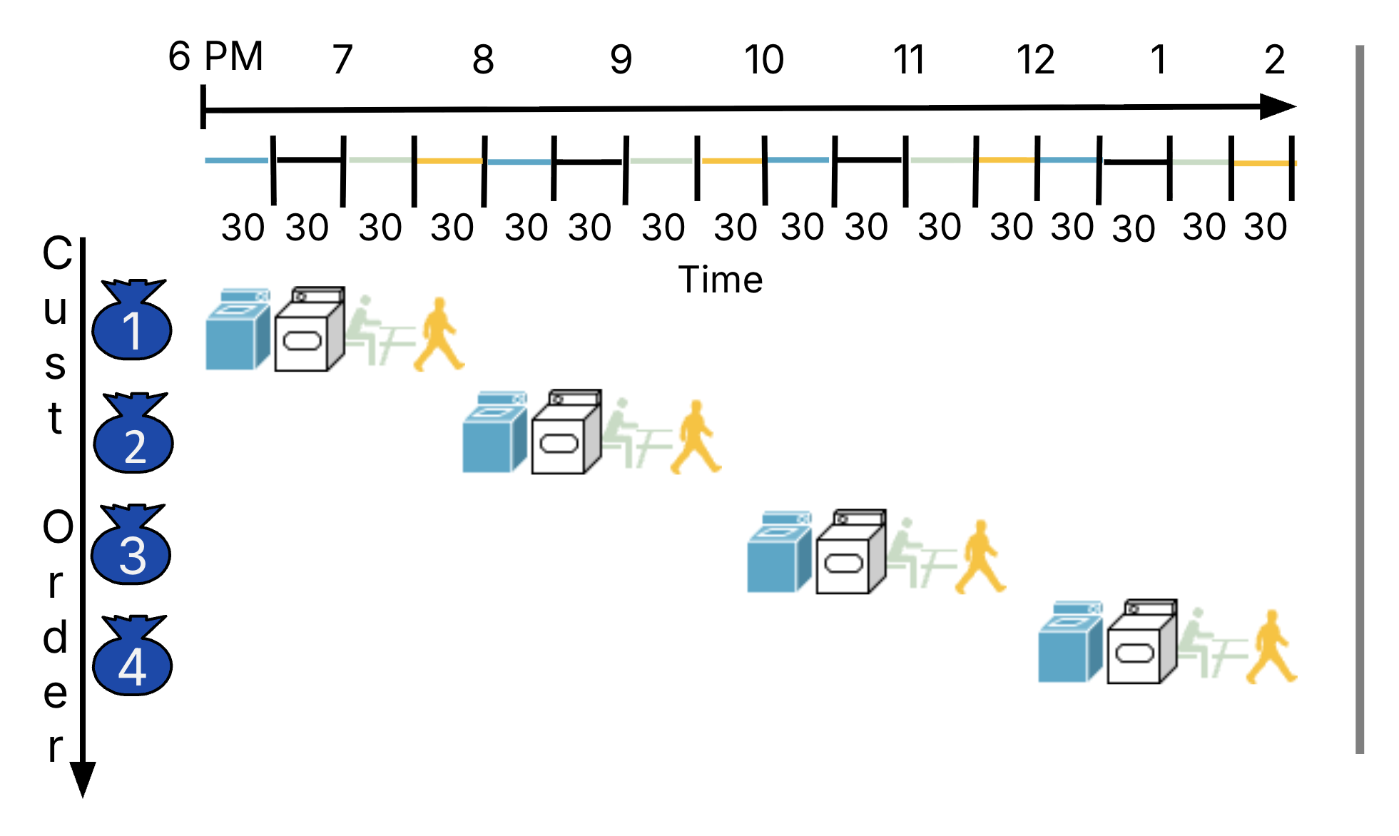
Figure 2:Timeline for sequential laundry.
This implementation takes 8 hours for just 4 loads of laundry. If we look closely at the four major resources, they are mostly wasted; after all, each person exclusively uses one of the washer, dryer, counter, and drawers as they are progressing through the four steps. The washer, for example, was only used for 30 minutes of the whole two hours.
We can certainly do better by trying to perform these steps concurrently, where each person performs a different step. This is the intuition behind pipelining.
3Pipelined Laundry
Now consider a pipelined approach to using laundry,[3] where as soon as Person 1 is done with the washer and takes out their wet clothes to move to the dryer, Person 2 can put their own dirty clothes in the washer, and so on. In Figure 3, Person 1 still starts at 6pm and finishes at 8pm, but now Person 4 can start much earlier at 7:30pm and finish by 9:30pm. Phew!
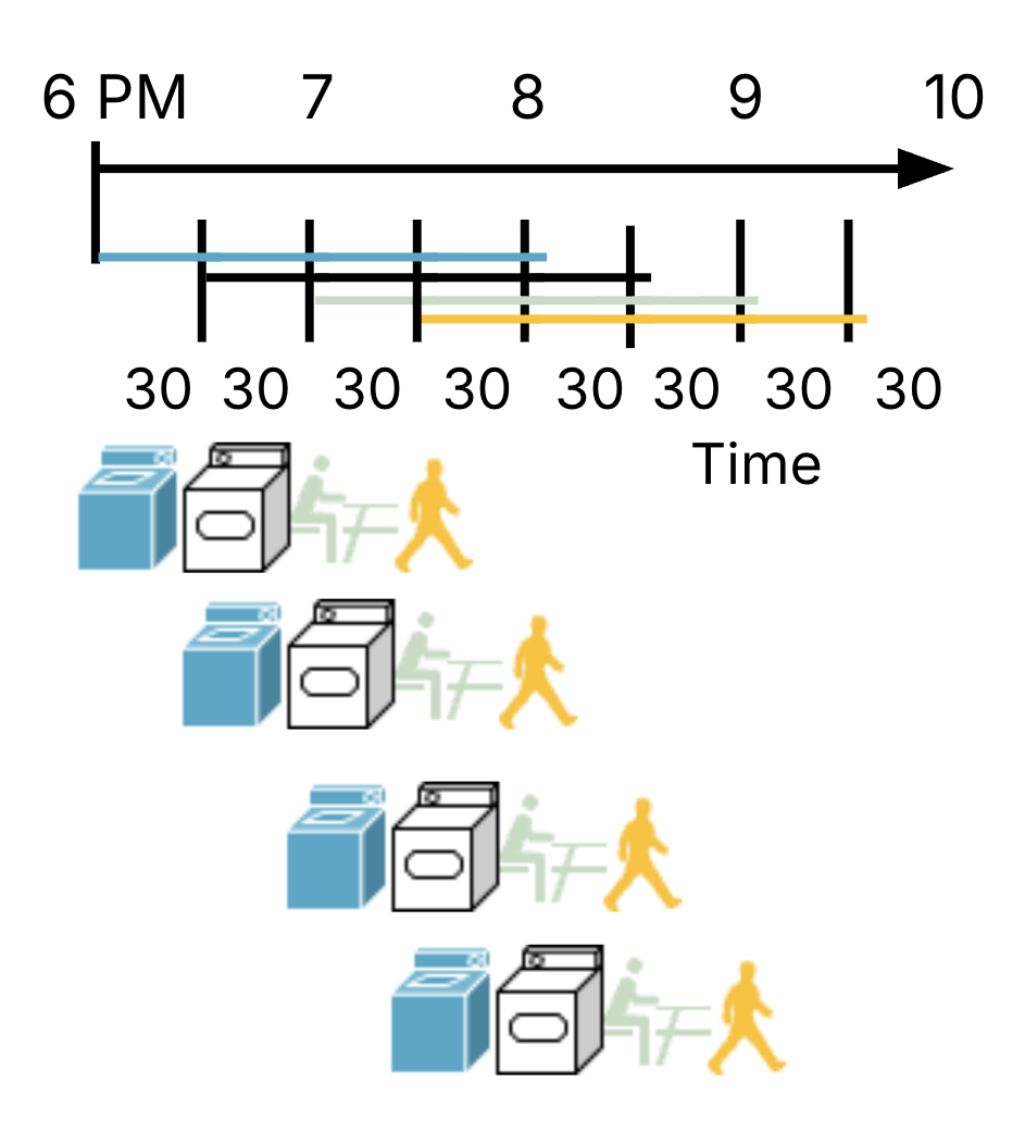
Figure 3:Timeline for pipelined laundry.
This implementation takes just 3.5 hours for the same 4 loads of laundry. At different 30-minute intervals, customers share the four resources because they are completing different steps of their laundry routine (Figure 4). At 7:30-8pm, all four resources are occupied by customers.
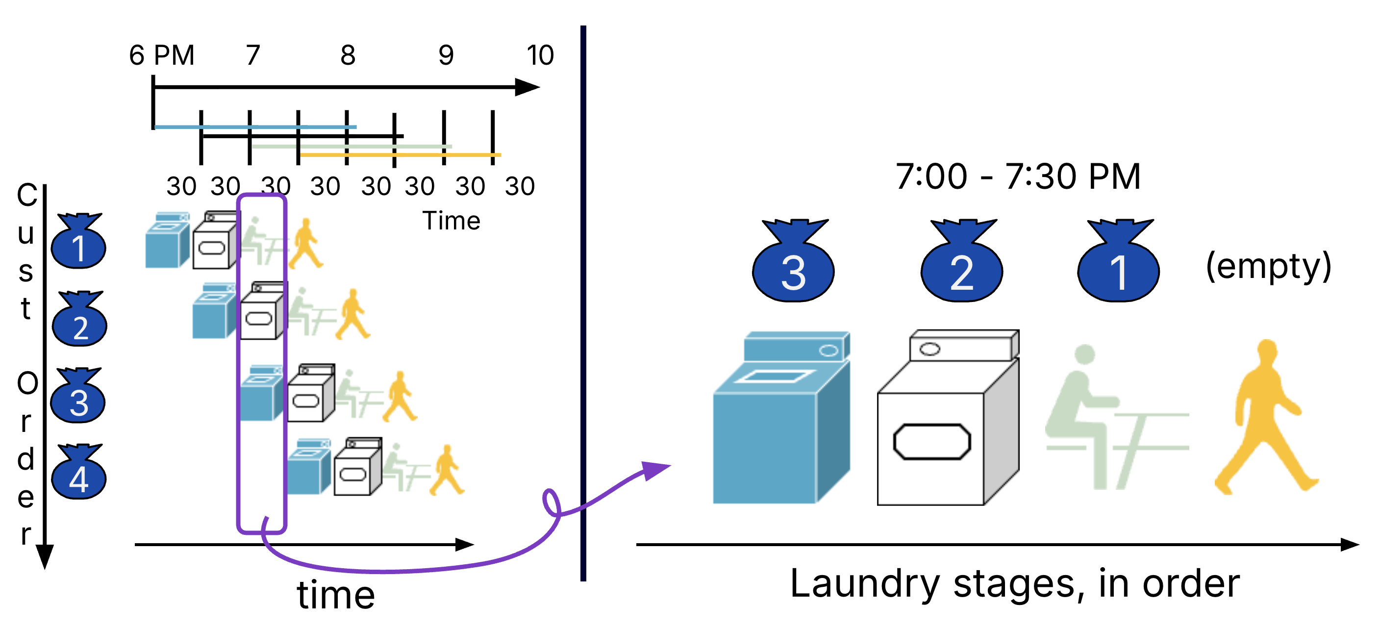
Figure 4:Two views of pipelined laundry: Over time (left) versus the snapshot of the laundry room during a given time interval (e.g., 7-7:30pm).
4Laundry: Latency vs. Throughput
From P&H 4.6:
The pipelining paradox is that the time from placing a single dirty sock in the washer until it is dried, folded, and put way is not shorter for pipelining; the reason pipelining is faster for many loads is that everything is working in parallel, so more loads are finished per hour. Pipelining improves *throughput* of our laundry system. Hence, pipelining would not decrease the time to complete one load of laundry, but when we have many loads of laundry to do, the improvement in throughput decreases the total time to complete the work.
Table 1 shows performance measures on our laundry benchmark task:
Table 1:Latency vs. Throughput: Sequential vs. Parallel Laundry.
| Measure | Laundry Analogy | Sequential | Pipelined |
|---|---|---|---|
| Program execution time | Time to finish all 4 loads | 8 hours | 3.5 hours |
| Instruction latency | Time to finish a single load | 2 hours | 2 hours |
| Instruction throughput | Average* number of loads per 30 mins | 0.25 | 1* |
Note (*): Throughput is approximate for our tiny 4-customer task. In this case, 4 loads complete in seven 30-minute intervals, or approximately 0.57 loads per 30-minute interval. If we had many customers, though, the pipeline is fully “filled,” where exactly 1 customer will finish each 30 minutes. We report this steady-state in the Table 1.
5RISC-V Processor: Sequential and Pipelined
Let us translate this laundry analogy back our RISC-V processor.
Consider how an instruction like add t0 t1 t2 accesses the hardware in the single-cycle processor. Like when we computed instruction timing, Figure 5 represents the five phases[4] with its major hardware unit.
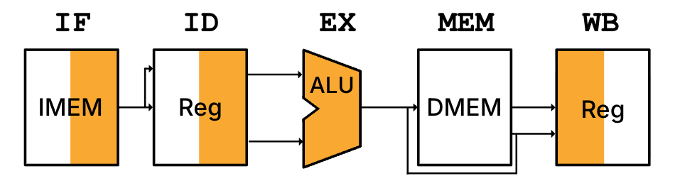
Figure 5:High-level diagram of single-cycle processor executing the instruction add t0 t1 t2. We adopt a graphic representation of each of the five phases, where each symbol represents the major hardware resource accessed in that phase. The shading illustrates if the unit is read (i.e., the right half is shaded for IMEM in IF and RegFile in ID) or the unit is written (i.e., the left half is shaded for RegFile in WB). For R-Type instructions, MEM is transparent because add does not access the data memory.
Suppose we use the single-cycle processor to execute three instructions, in sequence.
add t0 t1 t2
or  t3 t4 t5
lw  t6 8(t7)
In our single-cycle CPU, only one instruction can access any resources in one clock cycle, in sequence. As in Figure 6, executing these three instructions will take time, where .
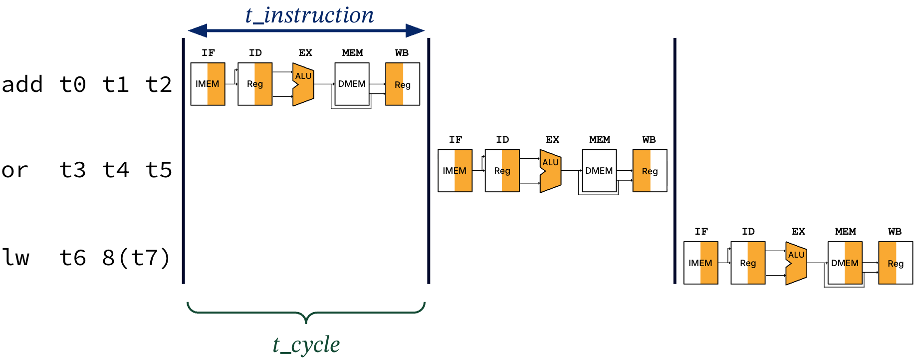
Figure 6:Single-cycle processor usage for three instructions. The instruction time is equal to the length of one clock cycle, .
In a pipelined processor, on the other hand, multiple instructions access different resources in a single cycle. Following our laundry analogy, we would like to design a pipelined processor that can produce the following timeline in Figure 7.
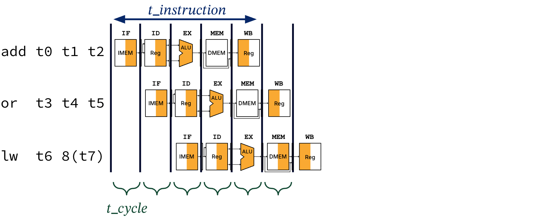
Figure 7:Pipelined RISC-V processor usage for three instructions. In the first cycle, add is in the IF stage. In the second cycle, or is in the IF stage, while add has moved onto the ID stage. In the third cycle, lw is in the IF stage, while or and add have moved onto the ID and EX stages, respectively. Each instruction now takes five cycles to execute, but the clock cycle can be timed to the duration of the longest stage.
If we examine our add t0 t1 t2 instruction and how it accesses the pipelined processor, we observe something like Figure 8.
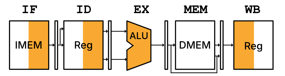
Figure 8:High-level diagram of pipelined processor executing the instruction add t0 t1 t2. Shading is described in the caption of Figure 5.
Notes:
We have pipeline registers separating each stage, meaning that each pipeline stage takes one clock cycle. We discuss this design in more detail in the next section.
The
addinstruction now takes five cycles to execute, so .The three instructions together now take time to execute.
Each cycle is much shorter, so the overall program execution time is shorter than the single-cycle processor.
All stages in the pipelined processor take the same length. Let us assume the same phase durations from the single-cycle processor as Table 2 from our instruction timing. In the pipeline, even though the hardware in the ID and WB stages may compute values faster, a singular clock means they will take as long as the other stages.
Table 2:Step timing: a phase in a single-cycle processor vs. a stage in the five-stage pipelined procssor. In the single-cycle processor, all five steps must occur in a single-cycle, so phase length is operation time. In the pipelined processor, each step is timed to the length of a stage, which must be the length of a clock period (because of pipeline registers).
| Step | Operation time | Single-cycle phase duration | Pipelined stage duration |
|---|---|---|---|
Instruction Fetch (IF) | 200 ps | 200 ps | 200 ps |
Instruction Decode (ID) | 100 ps | 100 ps | 200 ps |
Execute (EX) | 200ps | 200 ps | 200 ps |
Memory Access (MEM) | 200ps | 200 ps | 200 ps |
Write Back (WB) | 100ps | 100 ps | 200 ps |
Let’s compare this performance in Table 3.
Table 3:Performance comparison: Single-cycle processor vs. 5-stage pipelined processor.
| Comparison | Sequential | Pipelined |
|---|---|---|
| High-level diagram | INSERT | INSERT |
| Step timing | (see Table 2) 200 ps ( IF, EX, MEM); 100 ps (ID, WB) | 200 ps (all stages same length) |
| Clock period, | 200 + 100 + 200 + 200 + 100 = 800 ps | 200 ps |
| Instruction latency | = 800 ps | = 1000 ps |
| Clock frequency | 1/800 ps = 1.25 GHz | 1/200 ps = 5 GHz |
5.1Pipeline speedup
Based on Table 3, our throughput gain, or pipelining speedup, is close to the ratio of times between instructions. One approachis to time the single-cycle and pipelined processors against a benchmark program like 1 million lw instructions[5]:
The single-cycle processor takes = 800,000,000 ps.
The pipelined processor takes = 200,000,800 ps, where there are four cycles to accommodate the “startup” time of the pipeline (where not all stages of pipeline are used).
If we take the ratio of total execution times:
5.2Waterfall diagrams
Instead of repeatedly drawing the same tiny diagram as in Figure 7, we will use Table 4 to illustrate instruction execution in pipelined processors. This waterfall diagram should be read left-to-right: the leftmost column is the RISC-V instruction; all other columns are indexed by their time step (clock cycle, starting from 1). For each row, an entry in a time step column indicates the stage that the instruction is currently executing, or blank otherwise. For simplicity, we write MEM as M.
Instruction | 1 | 2 | 3 | 4 | 5 | 6 | |
|---|---|---|---|---|---|---|---|
| IF | ID | EX | M | WB | ||
| IF | ID | EX | M | WB | ||
| IF | ID | EX | M | WB |
The shared laundry room has a single washer, a single dryer, a single folding counter, and infinite but single set of drawers mysteriously located in the room itself.
Imagine there is a single key for the shared laundry room. At the beginning of the washing stage, you instantaneously obtain the key, unlock the room and enter, and relock the room so no one else can enter. Then right at the end of the folding stage, you instantaneously unlock the room, exit and relock, and put back the key.
Assume the door is unlocked now. The laundromat owner figured it out.
We assume no load data hazards in this program.