1Learning Outcomes
Use Amdahl’s Law to quantify the speedup to program execution time, given a specific optimization.
Use Amdahl’s Law to explain the limitations of infinite parallelization and the inherent bottleneck of non-parallel components.
🎥 Lecture Video
2Why parallelism?
To make a better computer and to run our applications faster, we have spent a good portion of time trying to understand the principles behind building a better computer. We have seen pipelining as a way to increase performance by working on multiple instructions at the same time in the pipeline.
Pipelining was the primary way people tried to increase processor performance from the 90s up to the early 2000s, where we kept building deeper and deeper pipelines and simultaneously used that to crank up the clock frequencies. However, as every processor generation came out, the power requirements kept shooting up—unsustainable, really (Figure 1). Eventually, Moore’s Law also tapered off.
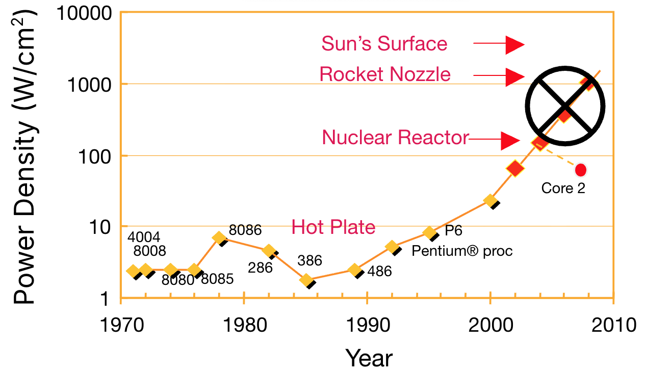
Figure 1:Power-Density prediction plot. Source: S. Borkar, Intel, circa 2000.
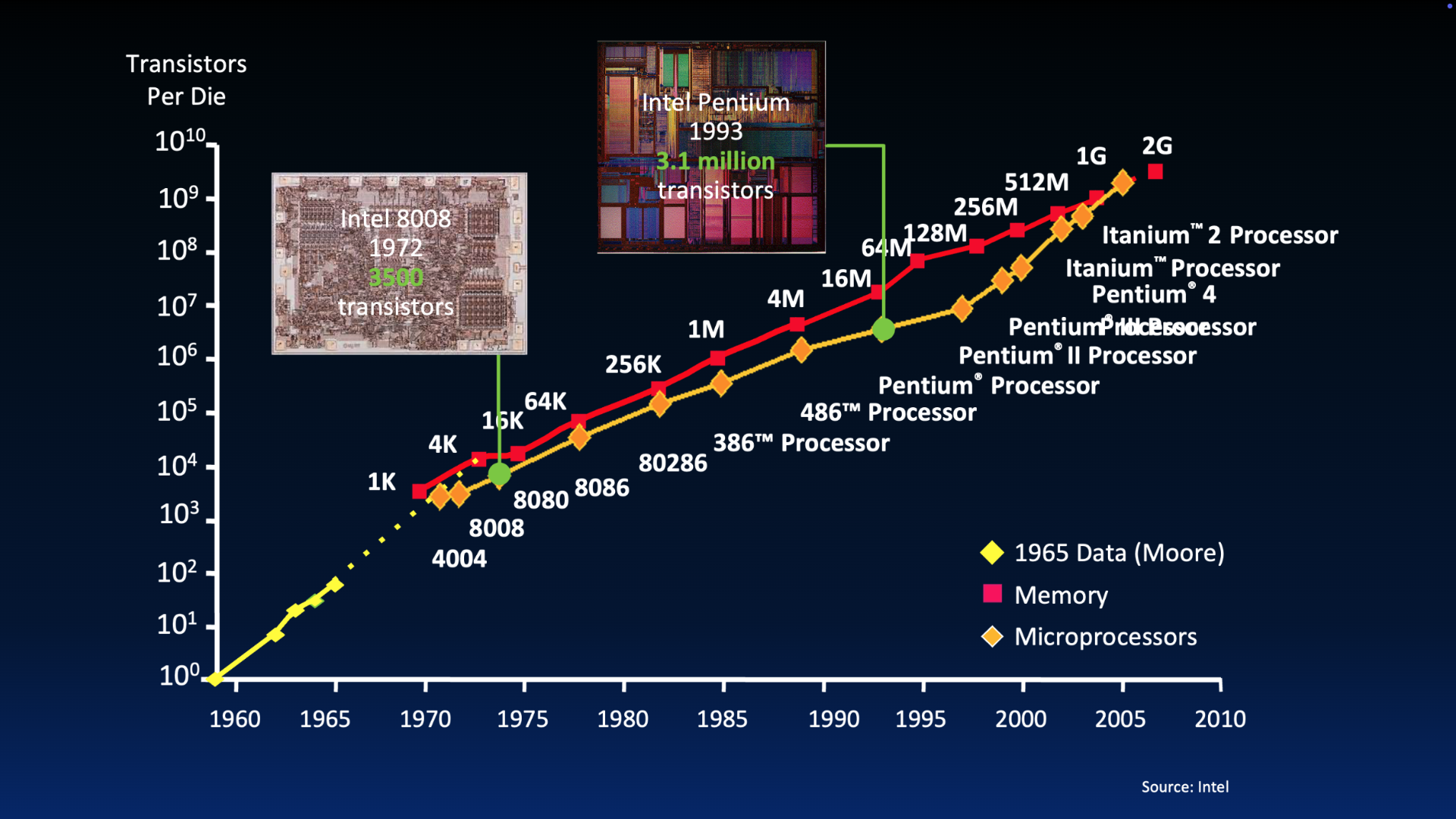
Figure 5:Visual of Moore’s Law over time.
To stay under reasonable power limits, people explored using parallelism in software and in hardware. Nowadays, almost all high-programs exploit parallelism in some way.
3Amdahl’s Law
A common pitfall when programmers first start pursuing performance (P&H 1.11):
Pitfall: Expecting the improvement of one aspect of a computer to increase overall performance by an amount proportional to the size of the improvement.
It reminds us that the opportunity for improvement is affected by how much fraction of time the improved event consumes.
Amdahl’s Law is the following straightforward Equation (1):
We rewrite Amdahl’s Law as Equation (2) to capture the speedup of a given program improvement, enhancement, or optimization:
Finally, we rewrite in terms of the proportion of the program that is optimized/affected by the improvement and the speedup factor to this component of the program to produce Equation (3):
Amdahl’s Law tells us that overall improvement to program execution time is not linear.
4Amdahl’s Law: Examples
The execution time of a third of a program can be accelerated by a factor of 2, due to some enhancement (e.g., multithreading and multicore).
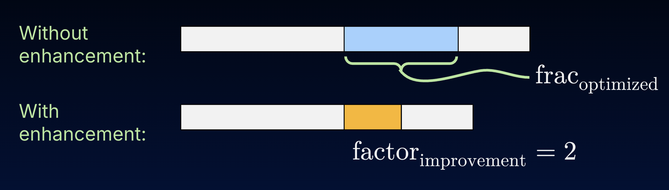
Figure 2:The execution time of a third of a program can be accelerated by a factor of 2 due to some enhancement.
The overall program speedup due to this enhancement can be computed using Amdahl’s Law (Equation (3)). Here, and .
Because parallelism is another type of program optimization, performance gains due to parallelism are limited by the ratio of software processing that must be executed sequentially. We illustrate this limitation below.
Show Answer
D. 9%.
One approach is to plug in choices until we exceed the desired 10x speedup with enhancement. We discuss this further below
5Parallelism: Theoretical limitations
Applications can almost never be completely parallelized; some code will always remain that must be executed sequentially.
As an analogy, consider Figure 4, where we collaborate with an infinitely large set of classmates to write a project report. In parallel, each classmate can do research and update a shared document, thanks to cloud technologies. However, even as the set of classmates approaches infinity, some fraction of the project will inevitably need to run sequentially before and after the large bulk of parallelization, e.g., to coordinate the parallel work itself, or to check for consistencies and print the report. These sequential parts may also increase and eventually outweigh any performance gains in parallelization.
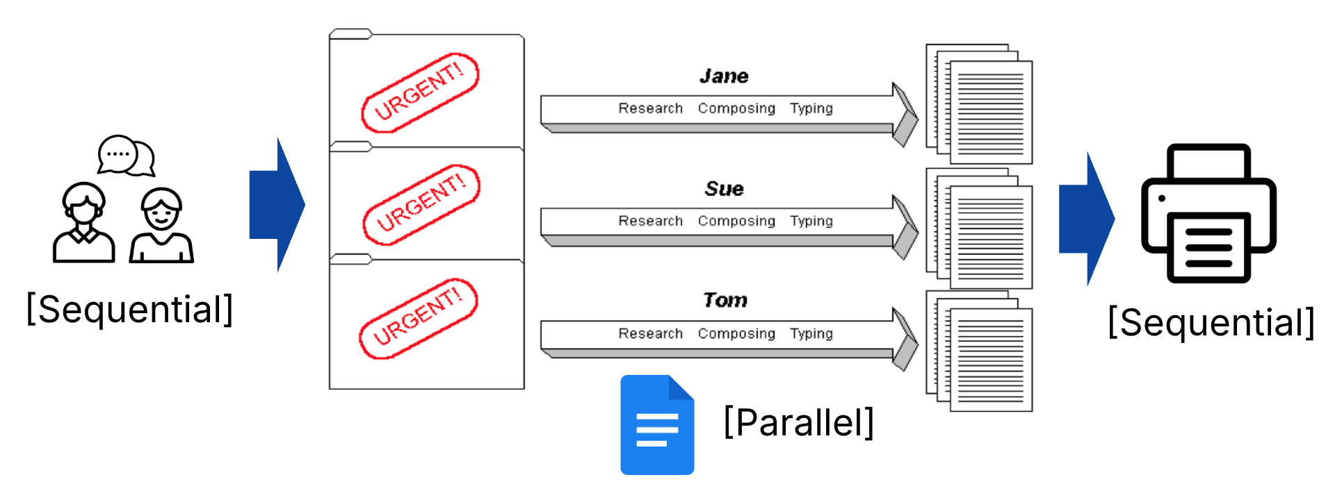
Figure 4:Reasonable assumption: Even with parallelization, some fraction of a program will need to run sequentially, e.g., to coordinate the parallel work itself.
In the simplest case, assume the parallelization speedup due to processors is . If we let be the sequential fraction of our program, then the eventual speedup is limited by :
In a perfect world, as the speedup factor goes to infinity—if you have a million or a trillion processors—the speedup can still be no bigger than than 1/s, determined by the sequential portion.[1] This theoretical limit is illustrated in Figure 5.
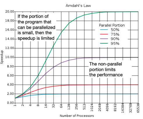
Figure 5:Plot of Amdahl’s Law: Speedup vs. Number of Processors.
Show Answer to Quick Check, continued
If we take a vertical line at 128 processors, we see that a 90% parallelizable program (e.g., 10% sequential) achieves less than a 10x speedup, whereas a 95% parallelizable program (e.g., 5% sequential) achieves more than a 16x speedup.
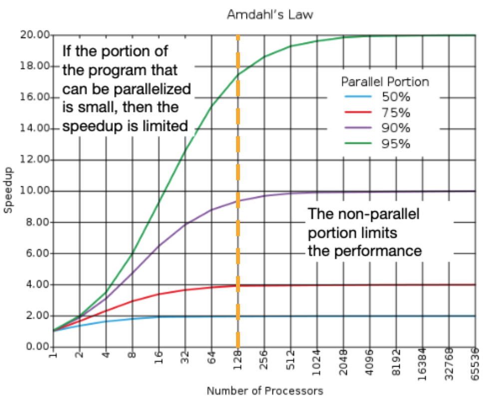
Figure 6:Consider the speedup described in the Quick Check.
Option D (9% sequential, or 91% parallel) is something in-between.
At the end of the day, parallelism in hardware does not solve everything. We will need to choose, design, and write software tasks that actually leverage the parallelism available in our architecture. Onto the next section!
Energy would also be a HUGE limitation here...!